Extracting Latent Dimensions Using Metric Unfolding

Multidimensional scaling (MDS) broadly speaking is a family of dimensionality reduction techniques which, given a dissimilarity matrix, produce a low-dimensional representation of the data which preserves the dissimilarities between points¹. MDS has applications in political science, with examples including the DW-NOMINATE model used by FiveThirtyEight and others to estimate the ideal points of US legislators² and its use by Hare et al. as a ‘hard test’ of the low-dimensional ideology hypothesis³. Political scientists have even developed Bayesian variants with the goal of obtaining accurate uncertainty estimates⁴.

MDS is a rich family of methods, and one of the particularly interesting variants for a political scientist is the broad sub-family of methods known as unfolding. In the unfolding setting, instead of our data being a square matrix expressing dissimilarities between units (e.g. between voters in terms of ideology, or legislators in terms of roll call patterns), we have a rectangular matrix. On our rows are judges or raters, and in each column is a particular stimulus to be rated. We wish to obtain a low-dimensional representation of the positions of both the stimuli and of the raters.

Numerous such datasets exist in political science and in particular in public opinion. One example is the ‘feeling thermometers’ in the American National Election Study (ANES)⁵. These are 0-100 scales where respondents are asked to express how ‘warm’ they feel towards particular stimuli, such as Donald Trump, Kamala Harris, the police, BLM, or the NRA. The thermometers have exactly the rectangular format just described, looking something like this:

My use of numbers ending in 0 and 5 isn’t accidental. While respondents can use the full range of numbers when responding, in the ANES data most opt for numbers ending 0, and a lesser number 5. Very few respondents offer other responses, though some do. As Jack Bailey has suggested on bluesky, this may be due to responding in person: respondents using online scales might have an easier time using other numbers⁶.

Questions of the usefulness of a 0-100 scale aside, this data is set up exactly as we would need it to be for unfolding. This is particularly attractive for a political scientist, because like (Bayesian) Aldrich-McKelvey scaling⁷, it enables us to obtain estimates of survey respondents and the stimuli they are rating on the same scale. Like other latent variable models and dimensionality reduction techniques such as PCA, factor analysis, and item response theory, interpretation of theis scale will depend on the data we put into the model and on qualitative inspection of the output.

In the remainder of this post, I’ll give a very brief primer on unfolding, before providing some examples via the ANES and British Election Study (BES) datasets.

Metric Unfolding

In classical, metric MDS, we are searching for a configuration of points such that the euclidean distances between embedded points \(\hat{d}_{ij}\) matches the input dissimilarties \(\delta_{ij}\) as closely as possible. We seek in particular to minimise the stress function:

In nonmetric MDS, we are instead minimising a stress function that seeks to preserve the montonic relationship expressed in the dissimilarities. That is, we are treating the dissimilarities as ordinal: we are preserving the rank order of the dissimilarities, but not their absolute values:

Where \(f\) is a montonically increasing function. Since we need to solve for both the points and to find \(f\), nonmetric MDS is often estimated iteratively, switching between finding \(f\) and updating the output configuration.

In the unfolding setting, we have a rectangular matrix with \(N\) respondents and \(M\) stimuli. We are seeking to minimise a stress function where we are finding a configuration of points for both stimuli and raters. In metric unfolding, this is given by:

There is a nonmetric variant of unfolding, but in this blog post I am restricting my attention to the simpler case. Before I proceed, it is worth noting that a whole universe of variants of the stress function exists, with a decent-sized and quite advanced literature on it. Suffice to say, for this blog post the main thing to understand is that we are finding a configuration of points which preserves some collection of dissimilarities.

SMACOF

Both MDS and unfolding models are most commonly estimated using SMACOF, which stands for Stress Majorization of a Complicated Function. Majorization is an approach to building optimisation algorithms wherein instead of directly optimising the function you would like to optimise, you find a surrogate function which is majorises that function and is easier to optimise. More plainly, given a function to be optimised \(f(x)\), we find an easier to optimise surrogate function \(g(x,y)\) for which the following majorization relationship holds:

where \(y\) is a fixed value called the supporting point. Additionally, the surrogate function must satisfy the relationship:

Intuitively, this property means that \(g(x,y)\) “touches” \(f(x)\) at \(x=y\), and otherwise is equal to or lies above it. To minimise the surrogate function in terms of \(x\), we find a new point \(x^*\) which satisfies the sandwich inequality:

This inequality ensures the new proposed value \(x^*\) does not increase the original function and so guarantees montonic improvement. Each new value further minimises both the surrogate, and by construction, the original function \(f\) - without ever needing to evaluate it. To iterate, set the value of \(y\) to be \(x^*\) and repeat the process of finding a new point. The resulting iterative procedure is:

1. Choose an initial starting value \(y := y_0\)
2. Find update \(x^{(t)}\) such that \(g(x^{(t)}, y) \le g(y,y)\)
3. Stop if \(f(y) - f(x^{(t)}) < \epsilon\) else set \(y := x^{(t)}\) and go to step 2

SMACOF is a particular implementation of majorization for the problems of MDS and unfolding. Happily for our purposes, it is implemented in the smacof⁸ R package with functions for both tasks. The unfolding function (also smacofRect) implements its namesake, and is very straightforward to use. I’ll now run through a few examples.

ANES Feeling Thermometers

For this example, I’m using the 2024 ANES dataset, and I’m using most of the post-election feeling thermometers in the dataset. I’ve avoided using the pre-election thermometers and some of the more relative post-election thermometers (e.g. senate candidates). I’ve recoded these in the dataset (see the bottom of this page just before footnotes for a link to full replication code for application of unfolding via SMACOF to the ANES feeling thermometers). The only important preprocessing step before beginning is to reverse the direction of the feeling thermometers, because when performing unfolding the function expects dissimilarities as input:

anes <- anes %>% filter(complete.cases(.)) # filtering missing data
therms <- anes |> select(-libcon_self) # used later on for visualisation
therms <- 100 - therms # reverse the direction

The exact dimensionality of the solution is chosen in advance by the practitioner. At times, 2 or 3 will be natural choices, as the goal will largely be to plot distance data and these are the maximum values for being able to do so. At other times there may be a good reason for choosing a particular value. However, in situations where there is an absence of such a priori criteria, such as this one, we can instead approach selection by producing a scree plot, much as we would in PCA. For this example I ran solutions up to 10 dimensions, including a progress bar in the code as this can be a little slow:

num_dims <- 10
pb <- txtProgressBar(min=0, max=num_dims, initial=0, style=3) 
smacof_models <- map(1:num_dims, function(x) {
  out <- unfolding(delta=therms, ndim=x)
  setTxtProgressBar(pb, x)
  return(out)
})

To produce a scree plot, we just plot the stress from each solution against the number of dimensions in the solution. Here are the results from the unfolding I ran:

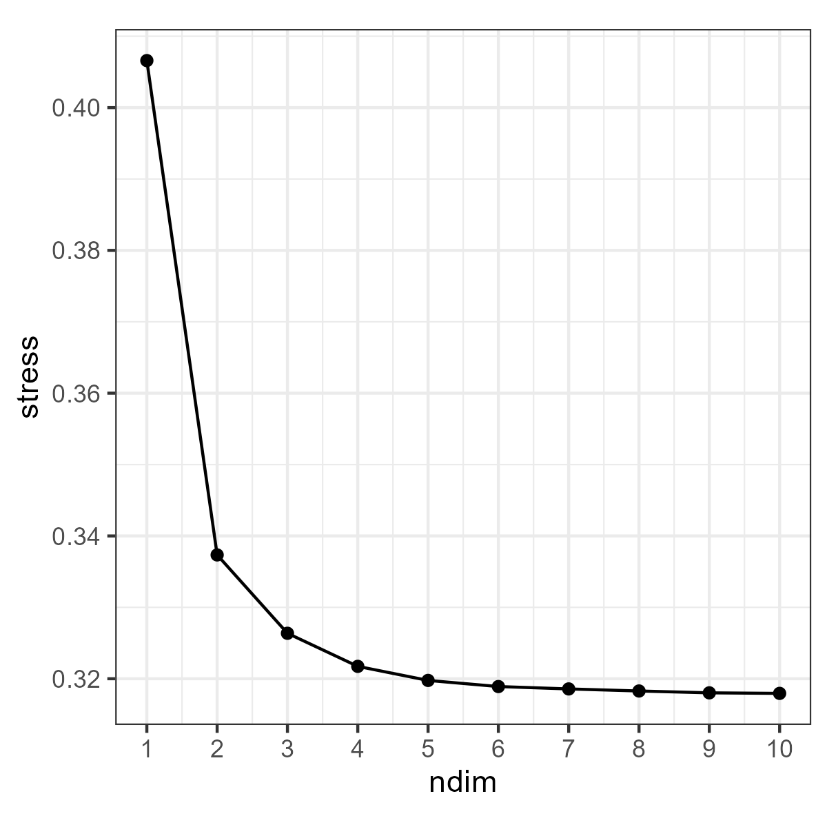
After reducing to 2 dimensions there are relatively few gains to be made by further increasing the number of dimensions in the solution and so I procceeded with the 2-dimensional configuration. With this configuration I have values in two dimensions for both the respondents placing the stimuli and the stimuli themselves. To inspect my solution I therefore plot both respondents and stimuli in a scatter plot, with the 1st dimension on the x-axis and the second dimension on the y-axis. I’ve plotted respondents as small, semi-transparent circles, coloured according to their self-placement on a 7 point liberal-conservative self-placement scale, with 1 being the most liberal and 7 the most conservative. I’ve plotted the stimuli as black triangles, with labels for all but the most overlapping stimuli. I’ve labelled the stimuli according to the text respondents are prompted with, rather than with the labels I would personally choose. This is how the configuration looks:

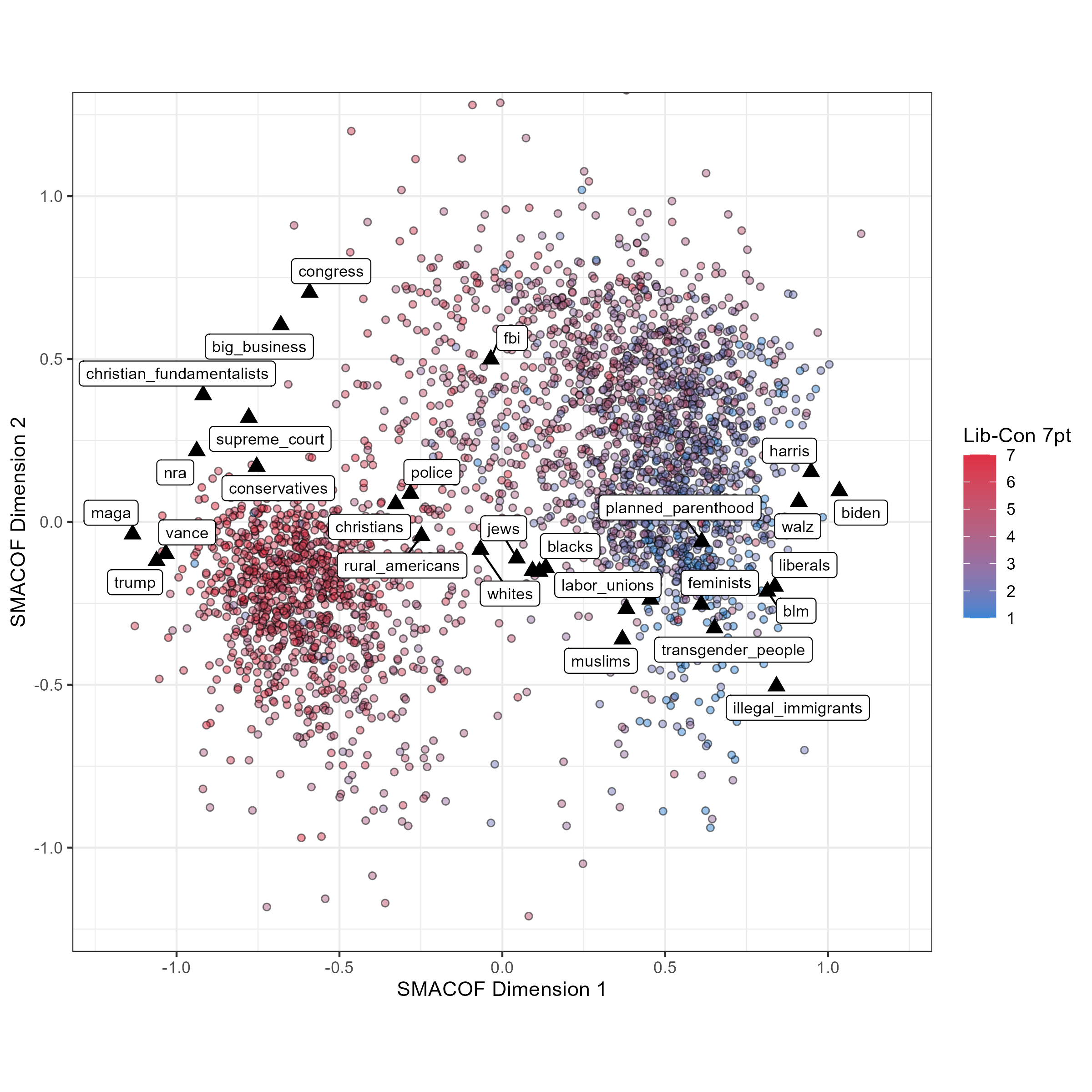
A solution such as this is best interepreted first in terms of the stimuli placements. On the 1st dimension, this seems roughly liberal-conservative, albeit it is an at least partially affective liberal-conservative dimension rather than a purely ideological one. I say so in part because the input data used is itself affective, but also because in the solution the most liberal stimulus is Joe Biden, whom can is generally understood to be a moderate Democrat. Trump’s placement would not be out of place in an ideological scale, but also largely reflects the affective dimension at play - we would expect him to be strongly disliked by liberal-minded respondents.

Most placements are largely as you’d expect on a dimension like this - the NRA, BLM, feminists, etc. Perhaps some of the more interesting ones are the racial and ethnic groups placed on the plot. They are typically middle-of-the-range, but with small differences that nonetheless reflect the racial politics of the US. The self-placements of respondents largely match the interpretation of the first dimension, and the pearson’s correlation between the first dimension and these self placements is -0.79, giving weight to the liberal-conservative interpretation.

The second dimesion in the output is harder to interpret. Solutions at times need to be rotated, though given the first dimension this does not seem to be the case here. It’s notable that high up on this dimension is the FBI, big business, and Congress, and that liberal respondents are typically higher on it than conservative respondents, although on the whole still more distant from these points. It could possibly reflect a sort of ‘establishment’ or ‘anti-establishment/populist’ dimension, but it isn’t easy to argue why trans people and Trump should end up roughly similar, or why given this interpretation Christian fundemantalists would also be high scoring.

All of this will reflect patterns in the thermometer ratings input into the data, but there are no guarantees the output dimension(s) will be straightforwardly interpretable. The liberal-conservative self-placement’s correlation with this dimension is much weaker, at -0.19, while the correlation of the two dimensions among respondents is 0.45. Interestingly, and reflecting the plot, among stimuli, the correlation between dimensions is reversed, at -0.49. I don’t quite know what to make of the fact that the stimuli appear to be misaligned from respondents on the second dimension, so will move on to the next example.

BES Like Scales

When I still did political science, my go-to dataset was (and remains) the British Election Study internet panel. It has a rich set of questions inside it, many of them potentially interesting to perform metric unfolding on. It’s therefore a natural choice for further examples in this blog post. I’m using the latest wave (30 at the time of writing), collected in May 2025, as a cross-sectional dataset⁹. For this example I use the ‘like’ ratings of parties and party leaders in the dataset, as the closest analogy to the feeling thermometers in the ANES. I restricted this to the five main GB parties, and I didn’t include the Green party leaders in the dataset as this rating has a much higher missing response rate.

The plot below is the output configuration from performing the same steps (albeit the output here was 3, rather than 2-dimensional). Unlike before, I haven’t scaled the x and y-axes to be the same. With apologies for the technical jargon, the shape of the output looks more like a rugby ball when scales are 1:1, but I found the spherical shape in this output nice to look at. The pleasure of writing blog posts is being able to be honest about this sort of reasoning. As before, I’ve plotted respodnents as circles, but coloured points according to their vote intention rather than their ideological self-placements.

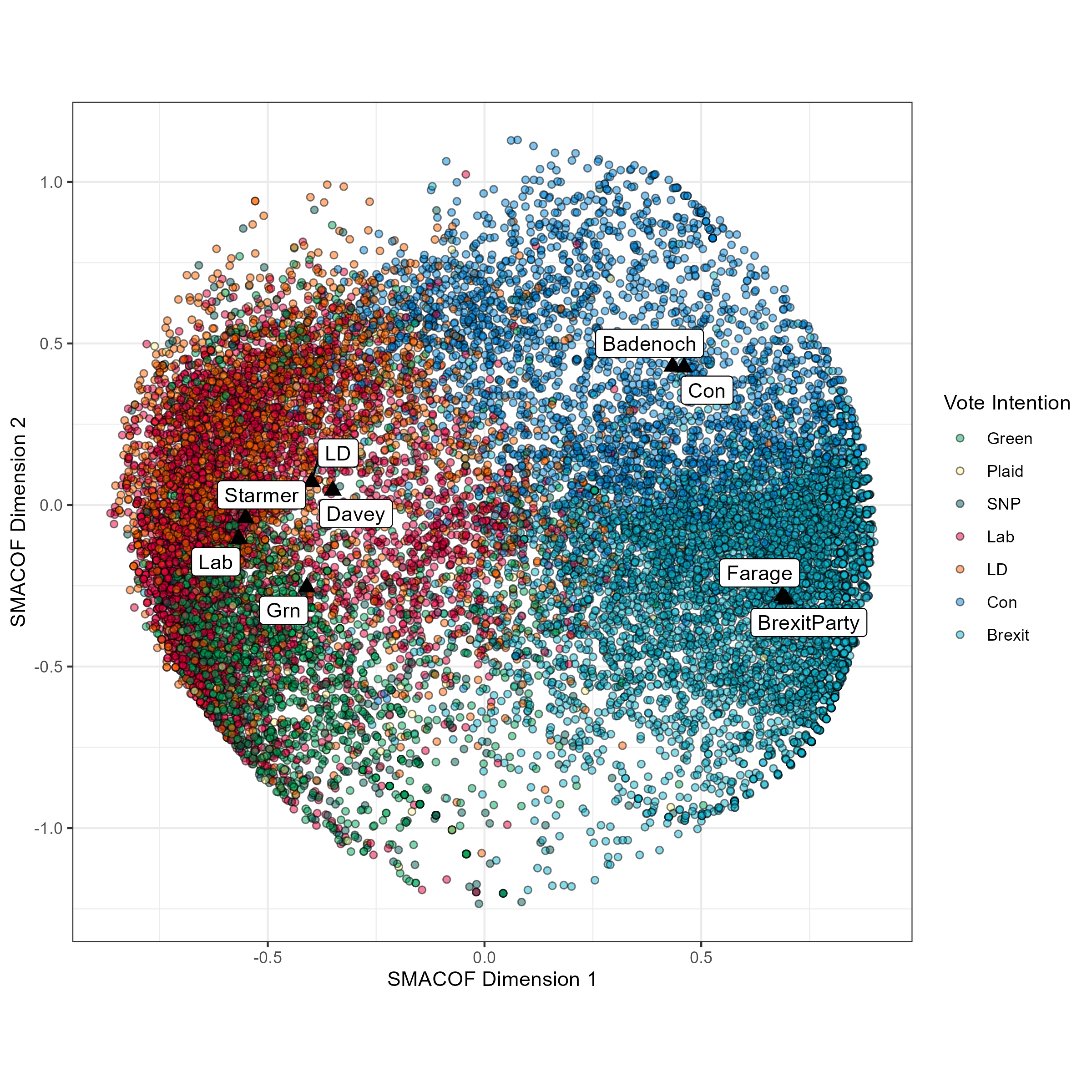
Starting once again with the first dimension, this seems as before an affective rather than pure left-right dimension. The biggest giveaway is the degree of distance between the left and right-wing stimuli, and the fact that Starmer and the Labour party came out to the left of the Greens. What’s perhaps more intersting is the proximity or distance of the respondents of various parties across both dimensions. In line with recent analyses¹⁰, voters of the three parties of the British left intermingle much more so than voters of the right-wing parties, and particularly so Labour and Liberal Democrat voters.

Reflecting the fact that their placements come from ‘like’ ratings, the stimuli likewise follow this pattern: the left-wing stimuli are clustered together, while the right-wing stimuli are far apart from one another. Unfolding the BES ‘like’ responses therefore allows us to reach a conclusion other analysts have reached using ideological data from the BES, which is that it is much harder to tell apart voters of the left parties than voters of the right parties.

The full code for running nonmetric unfolding using the smacof R package is available as a gist on github at this link. Note that you will need to download the ANES data yourself from this link and structure your working directory correctly.

Footnotes