Gradient Descent

According to Wikipedia, Gradient Descent is an iterative optimisation function for finding the local minimum of a differentiable function.

So what does all that actually mean?

Differential Functions and Local Minimums

It’s helpful to start at the end. Here, we’re using function in the mathematical sense of the term, which is something that given an input (e.g. a single number), produces an output (e.g. another number).

For example, we could use

\[ f(x) = x^2 \]

as our function. Or we could use

\[ g(y) = 5 + 2y^2 \]

as our function. The first takes an input \(x\), and squares it. The second takes an input \(y\), squares it, multiplies the result by two, then adds five to it.

Formally, a function assigns every element of a set \(X\) to a single output in the set \(Y\). Once this is set out, differentiable is clear: we can differentiate the function (i.e. establish a formula for the rate of change in the output).

The minimum of a function is the point at which the output is at its lowest possible value. For \(f(x)\) above, this is 0. For \(g(y)\), it’s 5.

Iterative Optimisation

An optimisation algorithm is one that finds the minimum or maximum of a given function. Sometimes, if a function is not convex, opitmisation algorithms may produce the local minimum or maximum instead of the true minimum or maximum. Often this depends on the starting value provided to the algorithm.

Iterative optimisation is then an algorithm that generates a sequence of improving approximations to the solution, where each iteration depends on the previous iteration.

Gradient Descent

Gradient descent is an iterative optimisation algorithm. It uses the first derivative to calculate an update for each iteration. Formally, given a function

\[ y = f(x) \]

the gradient descent update is given by

\[ x = x - \alpha \frac{\delta y}{\delta x} \]

where \(\alpha\) is a learning rate hyperparameter and \(\frac{\delta y}{\delta x}\) is the derivative of \(x\) with respect to \(y\).

When implementing Gradient Descent in practice, we also need two extra things. First, we want to set a maximum number of iterations. This is because without a maximum number gradient descent can just keep going and going. Second, we want to add a break condition. Eventually the changes will get so small as to be meaningless - so at this point we might as well stop instead of reaching the maximum number of iterations.

With all of this set out, we can now write our gradient descent algorithm:

import numpy as np

def gd(
    gradient_function: callable,
    start: float,
    learn_rate: float,
    max_iter: int = 100,
    tol: float=0.01
    ):
    """
    A simple implementation of gradient descent to optimise single-parameter functions

    Args:
        gradient_function: Callable for the gradient of the function being optimised
        start: Starting value to optimise from
        learn_rate: Learning rate for the update
        max_iter: Maximum number of iterations
        tol: Break clause for the gradient descent

    Returns: a dictionary containing the following:
        minimum: The estimated value at which the minimum of the function is found
        steps: Each step in estimating the minimum
        num_iter: The number of iterations
        final_diff: The final difference in estimated values
    """
    
    steps = [start] #tracking our steps
    minimum = start
    
    iter = 0
    diff = np.Inf
    while iter < max_iter and diff > tol:
        
        # Update
        minimum = minimum - learn_rate * gradient_function(minimum)
        
        # Store, increment, check diff
        steps.append(minimum)
        iter += 1
        diff = np.abs(steps[len(steps)-1] - minimum)
  
    # Store output
    out = {
        "minimum": minimum,
        "steps": steps,
        "num_iter": iter,
        "final_diff": diff
    }
    
    return out

An Example

To see Gradient Descent in practice, let’s consider the example of the following quadratic function:

\[ x^2 - 4x + 1 \]

It’s helpful to see a plot of what this function looks like:

import matplotlib.pyplot as plt

# The function we're considering
def quadratic(x):
    return x**2 - 4*x + 1

# 100 linearly spaced numbers
x = np.linspace(-5,5,100)

# apply the function
y = quadratic(x)

# setting the axes at the centre
fig = plt.figure()
ax = fig.add_subplot(1, 1, 1)
ax.spines['left'].set_position('center')
ax.spines['bottom'].set_position('zero')
ax.spines['right'].set_color('none')
ax.spines['top'].set_color('none')
ax.xaxis.set_ticks_position('bottom')
ax.yaxis.set_ticks_position('left')

# plot the function
plt.plot(x,y, 'r')

# show the plot
plt.show()

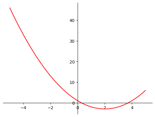
By the looks of things, the minimum of this function is around two (it won’t always be so easy though!).

The derivative of this function is given by

\[ 2x - 4 \]

So, let’s find the minumum of this function by using our gradient descent algorithm from above:

def quadratic_gradient(x):
    return 2*x - 4

est = gd(quadratic_gradient, start=9, learn_rate=0.5)
print(est["minimum"])

2.0

It worked!

Final Comments

The example above is nice for illustrating gradient descent, both because it has a single variable and because it has an obvious minimum that allows us to verify that gradient descent is doing what it’s supposed to be doing.

It’s worth stopping for a moment though to consider some more complicated cases.

First, let’s consider the case where we have a function of many variables, say

\[ y = f(x,u,v) \]

In this case, the gradient descent update for a parameter \(x\) is based on the partial derivative of \(y\) with respect to \(x\):

\[ x = x - \alpha \frac{\partial y}{\partial x} \]